Impacts of the Packing Plant Fire in Kansas
TOPICS
USDAMichael Nepveux
Economist

photo credit: Right Eye Digital, Used with Permission
Michael Nepveux
Economist
On August 9 a fire broke out at one of the largest beef packing plants in the U.S., significantly impacting beef markets in the days and weeks that followed. The fire, at a plant in Holcomb, Kansas, owned by Tyson Fresh Meats, stressed an already sensitive balance between processing capacity and a growing fed cattle supply. Immediately after the fire, the Holcomb facility’s cattle were sent to other facilities in an industry already facing a relatively strained capacity. Among the many questions surrounding the fire are how is it impacting stakeholders who both sell to and buy from this increasingly concentrated industry, and when we can expect everything to get back to normal?
How Big is the Plant and What’s Going on There?
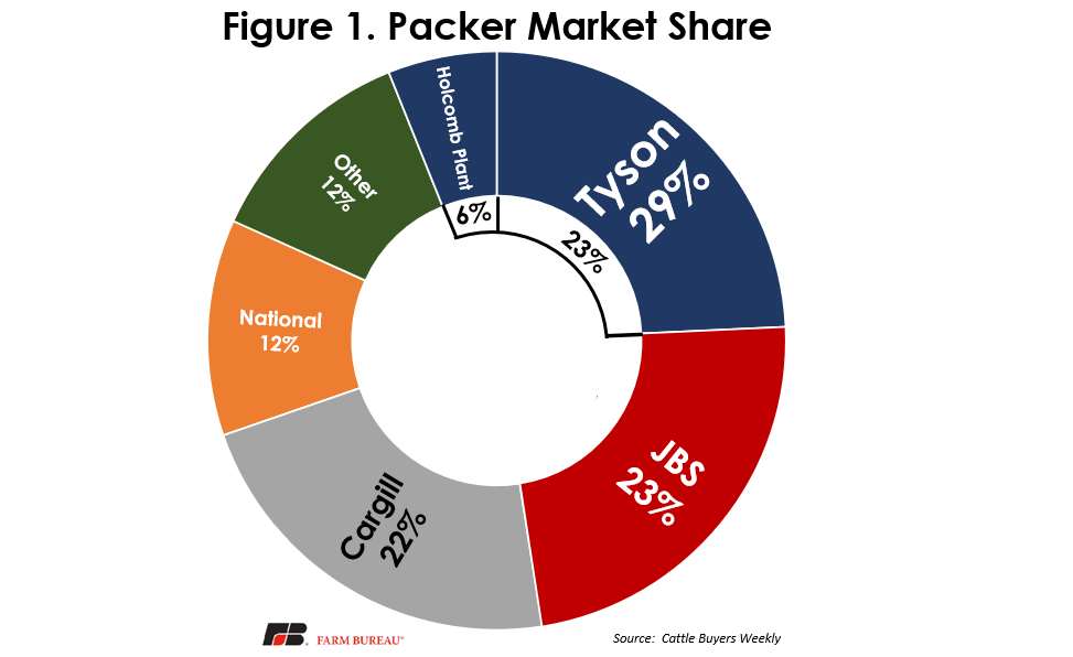
According to CattleFax, the Holcomb facility had a daily capacity of approximately 6,000 head, and accounted for about 6% of U.S. slaughter capacity, a not insignificant share for a single plant. Prior to the fire, Tyson held the nation’s largest market share of beef processing capacity at 29%, followed by JBS, Cargill and National at 23%, 22% and 12%, respectively. While the plant is out of commission, Tyson’s share could have dropped to 23%, however, due to reshuffling fed cattle to other facilities, Tyson will be able to keep the fire’s impact to its overall volume somewhat muted.
Nobody was hurt or injured during the fire, and first responders succeeded in putting it out before it spread to the rest of the plant. The majority of the damage was on the electrical system of the plant which is, as one would imagine, an extremely complex item to fix. Tyson still has not released an official timeline for plant repairs or set expectations for when it will be back on line. In the weeks following the fire, Tyson said the plant will be closed indefinitely until repairs can be made. However, in a recent investor call, representatives from Tyson said that it anticipates the plant to be fully back on line “in the course of the next couple of months,” and that they “expect the issue to be behind us and resume business as usual” by the new year. In the meantime, the company will continue to pay its hourly workers a full workweek wage.
What Would Economic Theory Tell Us Would Happen?
Immediately after the plant fire, we saw significant price movements in both the beef cutout, the product being produced by the packing plant, and in fed and feeder cattle, immediate and eventual inputs into the plant. The question is: is this what one would expect to happen under normal economic circumstances. The following graphic walks through a (very simplified) supply and demand response to the event, as well as the expected price response.

First, we should examine the situation before the fire, which is where the animation starts. On the right graph, we have a downward sloping demand curve (DemandB), which represents restaurant and grocery store demand for wholesale beef. On the same graph we have the upward sloping supply curve (SupplyB), which represents the beef that packers process and supply to the market. Where these two curves intersect results in the market equilibrium price of beef, denoted by PriceB. On the left side of the graph we have a similar set up for fed cattle, the major input for packers. Because packers require fed cattle to process into beef to supply their customers, we can develop a derived demand curve for fed cattle (DemandC). Feedlots and other cattle producers supply cattle to the market, resulting in the supply curve (SupplyC). Similar to the beef market, where these two curves intersect results in the market equilibrium price for fed cattle, PriceC. The difference between the price of beef and the price of cattle can be considered a (simplified) representation of the packer’s margin (not including processing costs, fixed costs, overhead, etc.).
The fire at the Holcomb facility was an exogenous shock to both the wholesale beef market and the fed cattle (and later down the supply chain, feeder cattle) market. In the beef market, this means the packing industry can supply less beef (assuming they were operating at capacity) to its customers, which is shown by shifting the supply curve inward and to the left (SupplyB-1). This shift results in a new higher equilibrium price (PriceB-1), as the supply has reduced while demand for beef has stayed the same (ceteris paribus). At the same time, since the packing industry has potentially lost 6% of its capacity, the industry is going to demand less of its input, fed cattle. This results in a leftward shift of the demand curve for cattle (DemandC-1), which in turn leads to a decrease in the equilibrium price for cattle (PriceC-1). With price for the input declining, and price for the output increasing, the remaining facilities that process cattle into beef would expect to see their gross margin increase, at least in the short run. Now that we have had some time to gather and process data, we can examine if what happened in the real world parallels economic theory.
Price Impact for beef
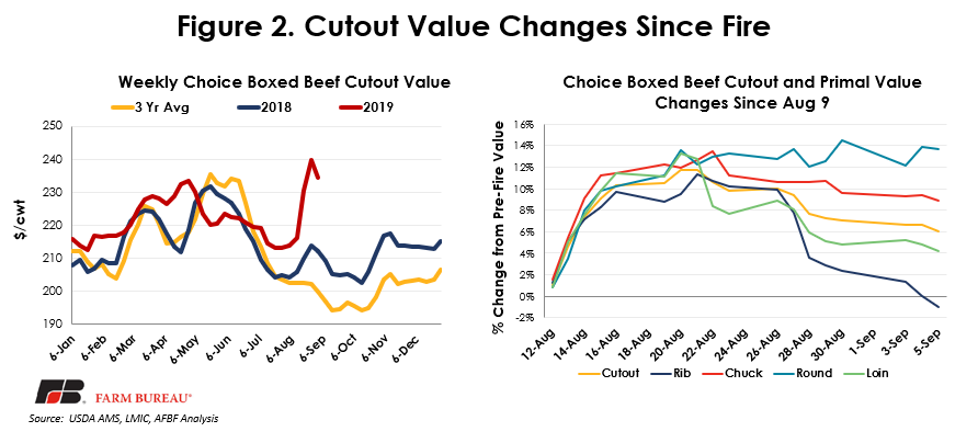
In the weeks following the fire, boxed beef values skyrocketed, moving from $216.04/cwt the week of the fire to $230.43/cwt the week after the fire and to $239.87/cwt the week after that. That’s a $23.83 jump in the two weeks after the fire. Downward pressure kicked in the third week after the fire and the cutout fell slightly to $234.35/cwt.
This pullback in prices has been mostly reflected across the primal values, but to differing degrees, as shown in Figure 2. Middle meats spiked immediately following the fire, and have since largely receded in value, with the rib dropping back down to pre-fire levels and the loin dropping to a 4% increase from its high of a 13% increase. End meats have managed to mostly sustain their higher levels since the fire, with the chuck and round remaining at or near a 10% increase from pre-fire levels. This is exactly the kind of market reaction one would have expected (at least directionally) from our basic analysis.
Price impact for cattle
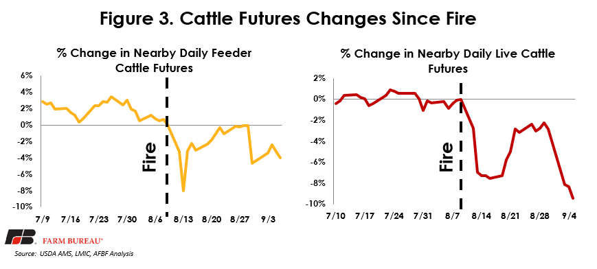
While the price of the beef cutout moved significantly upward, the fed and feeder cattle markets went in the opposite direction. Figure 3 examines the immediate impact the fire had on futures markets for the nearby daily feeder cattle futures contract and the nearby daily live cattle futures contract. It shows all prices as a percentage of the prices the day of the fire. For the month leading up to the fire, both feeder and fed cattle futures were largely holding steady at or slightly above the value the day of the fire. Immediately following the fire, both futures markets exhibited significant bearish activity. Though both markets recovered a bit in the days following the fire, those gains have since been muted. This market has experienced significant volatility following the fire. However, the initial downward movement of prices is what we would have expected based on our simple modeling above.
Slaughter Data
While the price movements were along the lines we expected, all of this activity falls under a key economic term, “ceteris paribus,” which means “all else equal.” A big assumption in all of this is that the packing industry did in fact lose 6% of its capacity, which was reflected in an approximately equivalent decline in cattle slaughtered/quantity of beef produced. This is where it was useful to wait a few weeks to write this article as there is a lag in some very key data.
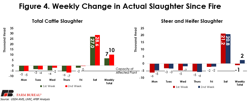
In the week following the fire, there were numerous reports in the marketplace that slaughter was actually up by 9,000 head of cattle, leading many industry participants to cry foul at the price movements. This doesn’t fully capture the whole story. Those numbers, while coming from a USDA report, were of estimated slaughter numbers, and were for total number of cattle. The report is the Estimated Daily Livestock Slaughter under Federal Inspection (SJ_LS710), and is an estimated early figure that is subject to revision. However, USDA’s Agricultural Marketing Service reports actual slaughter data under a two-week lag. This report is based on official Food Safety and Inspection Service data related to what was slaughtered. The report also shows a breakout of slaughtered steers and heifers, which we may be more interested in looking at instead of total cattle. So that means, we have two weeks of data after the fire occurred with which to compare results, which is shown in Figure 4.
We can see that the estimated slaughter number of 9,000 head was actually overstated, partly on larger estimated cattle and bull slaughter, and that actual total cattle slaughter for that week was up approximately 6,600 head for the week. However, it makes more sense to look at steer and heifer slaughter as opposed to total cattle slaughter in this instance. When looking at steer and heifer slaughter, we see that the first week after the fire, weekly slaughter was actually down around 1,000 head.
Another key takeaway is how close the daily slaughter for Monday through Friday was to the actual capacity of the closed plant (5,000 to 6,000 head). This tells us that many plants were already operating at or close to capacity prior to the Holcomb facility fire. However, with the economic incentive of increased margins, the processing industry will find a way to capture those margins, a fact reflected in the dramatic increase in weekend slaughter as facilities added extra shifts and shuffled cattle around plants.
Due to this additional slaughter on the weekend, the overall decrease in slaughter numbers is much smaller than we would have anticipated in our model. In fact, in the second week following the fire, the weekly numbers for steer and heifer slaughter actually increased, reflecting a rather quick adjustment on the part of the packers. Granted, this additional slaughter, which primarily occurred on weekends, is going to be in areas and shifts that are not as efficient, and so costs will likely be higher. Additionally, the transportation and other costs of shipping cattle that were going into the closed plant to other facilities further away will cut into those higher margins.
Margin impact for packers
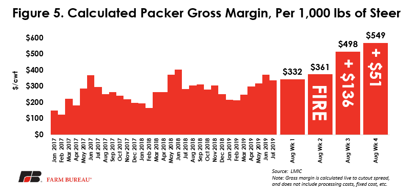
Packer margins significantly spiked following the increase in the beef cutout combined with the lower live prices, as the spread between live and cutout values subsequently widened. The Livestock Marketing Information Center does a great job of calculating packer gross margins on a 1,000 lbs.-of-steer basis. These calculations are essentially the spread between inputs and outputs, and do not include processing costs (energy, labor, etc.) and fixed costs. However, they still offer a good measure of the overall relative health of packer margins, and right now they are exceedingly healthy, as shown in Figure 5 with data current as of September 8. Leading up to the fire, calculated packer margins were healthy relative to the long run history. Since the fire we have seen historic levels of gross margins, at least in the 28 years this data has been collected. In the first week following the fire, gross margins jumped by $136 to $498, and in the following week they jumped an additional $51 to $549. Again, this is in line with what we would have expected. However, given that one of our major assumptions of declining beef supplies was negated by increased slaughter, this reminds us that real-world conditions rarely follow the assumptions in our neat economic models.
Following the price movements and the resulting margins, there was consternation from many in the cattle industry over the potential for some in the packing industry to take advantage of the situation and participate in unfair or illegal behavior. USDA took notice and announced that the secretary of agriculture was directing USDA’s Packers and Stockyards Division to launch an investigation “into recent beef pricing margins to determine if there is any evidence of price manipulation, collusion, restrictions of competition or other unfair practices.”
Summary
After the fire at the Holcomb facility, both the beef and cattle markets saw significant price movements, which led to historic gross margins for those involved in the beef packing industry. Much of this movement is right in line with what one would expect under these conditions, with the prices being driven by shifts in the demand curve for fed cattle and the supply curve for wholesale beef. However, a key assumption in these predictions is that actual slaughter numbers will fall relatively in line with the closed plant. Instead, we saw small decreases the following week, along with a small increase the second week after the fire as beef packers expanded weekend shifts to capture the additional margin being offered by the market. With the significant increase in volatility after the fire, and the concern by many in the industry for potential market manipulation, the American Farm Bureau Federation sent the following letter (Link) to USDA Under Secretary Greg Ibach on September 4, underscoring the importance of continuing to monitor the markets after such a market-moving event. Once again, this fire serves as a reminder that rarely do real world conditions perfectly align with the neat assumptions in our economic models.